
Latency & Response Time: Sub-Millisecond IO over 10 Million Requests
When your application communicates with a Brainboxes remote IO device over Ethernet, every command-and-response exchange takes time. This article explains what that response time means, why it matters for industrial IO and PLC applications, how to measure it accurately using HDR Histograms, and what results you can expect from Brainboxes devices.
What is Latency?
Think of latency like taking a bus to a destination. Your total journey time has two distinct parts: the time you spend waiting for the bus to arrive, and the time you spend travelling on the bus. Neither part alone tells you the full story -- your experience of the journey is the total of both combined. A fast bus is no use if you waited 30 minutes at the stop.
In the same way, when your application sends a command to a Brainboxes remote IO device, the total response time (or latency) includes:
- The time for your command to travel from your application, through the software stack, across the network, to the device
- The time for the device to process the command and interact with the IO hardware
- The time for the response to travel all the way back
The response time is the total round-trip time from the moment your application calls SendCommand() to the moment it receives the response.
Why Latency Matters for Industrial IO
Control Loop Timing
Industrial IO applications often run in tight control loops: read a sensor, make a decision, actuate an output. The response time of each IO operation directly limits how fast the control loop can run. A device that completes an IO round trip in 0.5 ms can theoretically support 2,000 control cycles per second.
Determinism and Predictability
For many industrial applications, it is not just the average response time that matters but the worst-case response time. A system that averages 1 ms but occasionally spikes to 500 ms may be unsuitable for safety-critical or time-sensitive applications. Predictable, bounded response times are essential.
PLC and SCADA Integration
When a Brainboxes device acts as remote IO for a PLC or SCADA system, the device's response time becomes part of the PLC's scan cycle. If the IO device responds slowly, the PLC must either extend its scan cycle or risk communication timeouts. Faster and more consistent IO response times allow tighter PLC scan cycles and more responsive control.
What Affects Response Time
A command travels through many layers on its way from your application to the IO hardware and back. Each layer adds time to the overall response.
| Segment | What Happens |
|---|---|
| Application layer | Your C# code calls ed.SendCommand() or reads ed.Inputs[0].Value |
| Software stack | .NET runtime serialises the call, OS TCP/IP stack builds packets, NIC driver queues them |
| PC NIC hardware | The Ethernet NIC transmits the packet onto the wire |
| Ethernet network | The packet travels through cables, switches, and routers |
| Brainboxes hardware | The device's Ethernet interface receives and buffers the packet |
| Brainboxes firmware | The command is parsed and the appropriate IO operation is executed |
| IO hardware | Physical reading of inputs or setting of outputs (relays, ADCs, DACs) |
| Return path | The response travels the same chain in reverse back to your application |
Returning to the Bus Analogy
Just as many factors affect a bus journey, many factors affect response time. Consider what can slow a bus down:
| Bus Journey | System Equivalent |
|---|---|
| Traffic lights and junctions | Network switches and routers -- each hop adds processing time |
| Road works | Network congestion, packet retransmissions, or TCP retries |
| Driver's familiarity with the route | Firmware optimisation and protocol efficiency on the device |
| Bus engine maintenance | Hardware condition -- NIC performance, cable quality |
| Time of day and busyness of roads | Network load -- other devices competing for bandwidth |
| Weather | Electromagnetic interference, environmental conditions affecting signal quality |
On a good day with clear roads, your bus arrives quickly and predictably. On a bad day, any single factor can slow the whole journey. The same applies to system latency: every component in the chain contributes, and any one of them can introduce delay.
The total response time is the sum of all these segments in both directions. In a well-configured test environment -- direct cable, static IP, no switches -- network latency is minimised, so the measured time primarily reflects the device's own processing and IO hardware performance.
Latency Does Not Follow a Normal Distribution
A common assumption is that if the average response time is 0.5 ms, most responses will be close to 0.5 ms, with a symmetrical spread above and below. This would be true if latency followed a normal (bell curve) distribution. But it does not.
  Normal Distribution                    Long-Tail Distribution (Latency)

        ▄███▄                            █
       ▐█████▌                           █▌
      ▐███████▌                          ██
     ▄█████████▄                         ██▌
   ▄█████████████▄                       ███
 ▄█████████████████▄                     ███▌
█████████████████████                    ████▄▃▂▁▁▁▁▁▁▁▁▁▁▁▁▁▁▁▁▁▁
─────────┼─────────                      ──────────────────────────────▶
      mean = median                      median    99%  99.99%     max
                                              ◀─ long tail ──────────▶
  Symmetrical: most values                Skewed: most values are fast,
  cluster around the mean                 but outliers can be 10-100x slower
In practice, latency distributions have long tails. The vast majority of responses are fast and tightly clustered, but a small number of outliers take much longer -- sometimes 10x, 50x, or even 100x slower than the median.
Why Outliers Matter
In an industrial system processing millions of IO operations, even a tiny percentage of slow responses can cause real problems. Consider: if 99.99% of responses complete in under 1 ms but the remaining 0.01% take 35 ms, that means every million operations includes about 100 operations that are 70 times slower than normal. For systems where every cycle must complete within a deadline, these outliers define the true worst-case behaviour of the system.
A small number of outliers often has a disproportionate effect on overall system performance. It is not the typical case that causes failures -- it is the exceptional one.
Mean and Standard Deviation Are Not Enough
Because the distribution is not normal, the mean and standard deviation do not give a useful picture of latency behaviour. What you need is a way to see the full percentile distribution -- especially at the extreme tail. You need to be able to answer questions like: "What response time did 99.99% of my requests complete within?" and "How bad is my worst 1-in-a-million case?"
For example, the ED-588 with a single connection shows a mean of 0.496 ms and a standard deviation of just 0.085 ms. These numbers suggest very tight, consistent performance. But looking deeper: 99.9% of requests complete within 0.645 ms, while at 99.999% (five nines) the latency jumps to 11 ms, and the absolute maximum across 10 million requests is 35 ms. The mean alone hides this 70x jump entirely.
The Compounding Effect of Latency
The tail latency problem gets worse when a system must make multiple requests to complete a single operation. The end user does not experience the median latency of an individual request -- they experience the worst request in the chain.
A Simple Example: 10 Friends Meeting for Coffee
Imagine 10 friends agree to meet at a coffee shop at 10am. Each takes a different bus, planning their journey based on the typical (median) travel time. They all expect to arrive right on time.
What are the chances all 10 arrive on time?
If each friend has a 95% chance of being on time -- a pretty good bus service -- the probability that all 10 arrive on time is:
0.95^10 = 59.9%
Nearly half the time, someone is late. Even with a 95% reliable journey, the group only has a 60% chance of all being there on time. With a more realistic 90% on-time rate per person, it drops to:
0.90^10 = 34.9%
Two times out of three, the group is waiting for someone. The group's experience is not the median -- it is dominated by the slowest individual.
How This Applies to Systems
Consider a system that must make 100 internal IO requests to present one complete result to the user. The user does not experience the median latency of a single request. They experience the worst of those 100 requests. If a typical user interaction involves viewing 5 such results, they are exposed to the worst of 500 individual requests. Most users will experience worse than the 99th percentile of individual request latency.
An Industrial Example
An industrial control system makes 50 remote IO requests per cycle and runs 2,000 cycles per day. That is 100,000 individual IO requests per day.
If 99.99% of requests complete within 1 ms but the remaining 0.01% take 35 ms, that means roughly 10 slow requests per day. For a factory operator who needs tasks to complete within tight time windows, experiencing a noticeable delay at least twice per day is almost certain.
The probability of seeing zero delays in a day:
0.9999^100,000 ≈ 0.005 -- less than 1%
This is why tail latency matters so much, and why measuring at the 99.99th percentile and beyond is not academic -- it is the reality your users and operators experience every day.
HDR Histogram: A Better Way to Measure Latency
HDR Histogram (High Dynamic Range Histogram) is a data structure designed by Gil Tene to record and analyse latency distributions with precision across a very wide range of values. Unlike a simple average or a standard histogram with fixed-width bins, an HDR Histogram preserves detail at every percentile -- from the median all the way out to the 99.9999th percentile and beyond.
This matters because it lets you answer the questions that actually determine system behaviour: not just "what is the average?", but "what response time did 99.99% of requests complete within?" and "how does my tail latency compare at different concurrency levels?"
Gil Tene's talk How NOT to Measure Latency is essential viewing for anyone working with latency-sensitive systems. It explains why common measurement approaches produce misleading results and how HDR Histograms solve the problem.
The HDR Histogram project provides implementations in many languages including C# (via the HdrHistogram NuGet package). Test results are saved as .hgrm files, which can be plotted interactively using the HdrHistogram online plotter.
How to Read an HDR Percentile Plot
HDR percentile plots have the percentile on the X-axis (scaled logarithmically toward 100%) and latency on the Y-axis. A flat horizontal line means consistent, predictable performance. An upward curve at the right-hand side reveals tail latency -- the behaviour of the slowest responses. The further right the line stays flat before curving up, the more "nines" of consistent performance the system delivers.
Brainboxes Response Time Performance
Brainboxes remote IO devices deliver robust, predictable response times to a very high number of nines. Here are the results from an ED-588 running the @AA command (read all digital IO line states) over the ASCII protocol:
| Concurrent Connections | Mean (ms) | 99th %ile (ms) | 99.99th %ile (ms) | Max (ms) | Total Requests |
|---|---|---|---|---|---|
| 1 | 0.496 | ~0.588 | ~0.866 | 35.123 | 10,000,000 |
| 2 | 0.642 | ~0.805 | ~10.758 | 11.053 | 100,000 |
| 4 | 1.292 | ~1.487 | ~25.843 | 41.677 | 100,000 |
| 8 | 2.487 | ~24.307 | ~79.360 | 99.277 | 100,000 |
Key observations:
- Sub-millisecond median: With a single connection, the median response time is 0.495 ms -- under half a millisecond.
- Extremely tight distribution: From the 50th to the 99th percentile, latency increases by only 0.093 ms (from 0.495 to 0.588 ms). 99 out of 100 requests complete within 19% of the median.
- Very high nines: At 99.9% (three nines), latency is still only 0.645 ms. At 99.99% (four nines), it is 0.866 ms -- still under 1 ms.
- Graceful concurrency scaling: With 2 concurrent connections, the mean rises to 0.642 ms (1.3x). With 4, it reaches 1.292 ms (2.6x). The near-linear scaling shows the device handles concurrent load predictably.
Test Setup
The results above were collected under controlled conditions designed to isolate the device's own response time performance.
- Software: C# test application using the Brainboxes.IO .NET API with the HdrHistogram NuGet package for latency recording.
- Network: The PC's Ethernet NIC is connected directly to the Brainboxes device with a single Ethernet cable. Both use static IP addresses. No switches, routers, or other network devices are in the path.
- Protocol: ASCII protocol on TCP port 9500.
- Timing resolution:
Stopwatch.GetTimestamp()provides 100-nanosecond resolution -- the highest available in .NET. - Test duration: The single-connection test runs 10 million iterations. Multi-connection tests run 100,000 iterations each. The 10 million iteration test provides extremely high precision at the tail percentiles.
The Test Code
The Brainboxes.IO .NET API is open source. You can download the code from GitHub and run these latency tests against your own Brainboxes devices using LatencyTestASCII.cs.
Here are the key portions that show how the measurements work.
Histogram Setup
// A Histogram covering the range from 1 tick (100ns) to 1 hour
// with a resolution of 3 significant figures:
var histogram = new LongConcurrentHistogram(1, TimeStamp.Hours(1), 3);
LongConcurrentHistogram is thread-safe, so it can be written to from multiple parallel connections simultaneously. The range covers 1 tick (100 ns) up to 1 hour, with 3 significant digits of precision -- meaning values are recorded with 0.1% accuracy across the entire range.
The Measurement Loop
(View on GitHub -- lines 221-254)
Parallel.For(0, parallelRequests, (p) =>
{
    EDDevice ed = new EDDevice(new TCPConnection(ip, port, 10000), new ASCIIProtocol());
    ed.Connect();
    for (int i = 0; i < requestsPerLoop; i++)
    {
        string newCommand = nextCommand();
        long startTimestamp = Stopwatch.GetTimestamp();
        ed.SendCommand(newCommand);
        long elapsed = Stopwatch.GetTimestamp() - startTimestamp;
        histogram.RecordValue(elapsed);
    }
    ed.Disconnect();
});
Each parallel connection creates its own EDDevice with a separate TCPConnection and ASCIIProtocol. The timing wraps only the SendCommand() call -- the full synchronous send-and-receive round trip. The elapsed time in ticks is recorded directly into the concurrent histogram.
Output
(View on GitHub -- lines 257-267)
histogram.OutputPercentileDistribution(
    writer: writer,
    outputValueUnitScalingRatio: OutputScalingFactor.TimeStampToMilliseconds);
string fileName = $"{deviceType}-{commandName}-{parallelRequests}x.hgrm";
File.WriteAllText(fileName, writer.ToString());
The histogram outputs its full percentile distribution with values scaled to milliseconds and writes the result to a .hgrm file. These files can be uploaded directly to the HdrHistogram online plotter for visualisation.
Command Generators
(View on GitHub -- full test file)
The test suite exercises several different ASCII commands:
| Test Method | Command | Description |
|---|---|---|
AtAALatencyTest | @AA | Read all digital IO line states |
AtAADDLatencyTest | @AA(Data) | Set digital outputs to random values |
HashAANLatencyTest | #AAN | Read digital input counter for a random channel |
AA1N0FLatencyTest | #AA1N0F | Set all 4 analog outputs to random voltages (ED-560) |
HashAA1NVVDataAnalogSetMultipleLines | #AA1NVVData | Set multiple analog output channels simultaneously |
Each command generator produces a new command string for every iteration. Commands that accept data parameters use random values to exercise different code paths on the device firmware.
Reading the Results
The .hgrm output files contain the full percentile distribution. Here is a condensed excerpt from [email protected] (10 million requests, single connection):
[email protected] -- percentile distribution (click to expand)
       Value     Percentile TotalCount 1/(1-Percentile)

       0.429 0.000000000000          1           1.00
       0.457 0.100000000000    1017078           1.11
       0.495 0.500000000000    5019833           2.00
       0.537 0.900000000000    9013591          10.00
       0.588 0.990625000000    9907099         106.67
       0.645 0.999023437500    9990355        1024.00
       0.866 0.999877929688    9998785        8192.00
      11.162 0.999992370605    9999924      131072.00
      35.123 0.999999904633   10000000    10485760.00
#[Mean    =        0.496, StdDeviation   =        0.085]
#[Max     =       35.123, Total count    =     10000000]
Each column tells you something specific:
| Column | Meaning |
|---|---|
| Value | The response time in milliseconds at this percentile |
| Percentile | The fraction of all requests that completed at or below this value |
| TotalCount | The cumulative number of requests at or below this value |
| 1/(1-Percentile) | The "one in N" ratio -- how many requests you would need to send before seeing one slower than this value. At the 99.9th percentile (1,024), one in every 1,024 requests exceeds 0.645 ms |
The HDR Histogram Graph
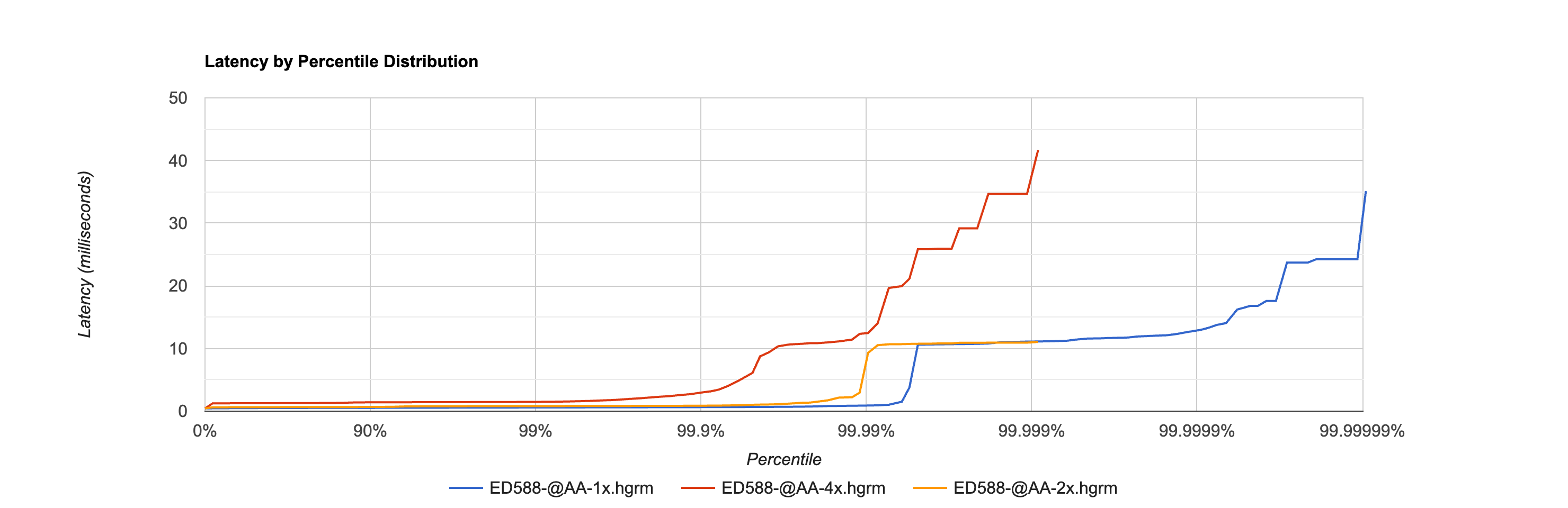
This graph shows the latency percentile distribution for the ED-588 @AA command with 1, 2, and 4 concurrent connections.
The X-axis shows the percentile on a logarithmic scale stretching from 0% to 99.99999%. The Y-axis shows latency in milliseconds.
Key observations:
- The 1x line (blue) stays flat near 0.5 ms for the first 99.99% of all requests, only rising at the extreme tail to reach 35 ms at the absolute maximum. This flatness demonstrates remarkably consistent performance across 10 million operations.
- The 2x line (orange) runs slightly higher (~0.6 ms) and also remains flat until the extreme tail, reaching ~11 ms.
- The 4x line (red) runs at ~1.3 ms and shows a more gradual rise starting around the 99th percentile, where contention between the four concurrent connections becomes visible.
- The fact that all three lines remain flat for so long -- well past 99% and even past 99.99% for the single connection case -- demonstrates the device's consistent and predictable performance under load.
Comparison to Other Industrial IO Systems
To put these results in context, here is how Brainboxes response times compare to other common industrial IO approaches:
| System Type | Typical Response Time | Notes |
|---|---|---|
| Brainboxes ED-588 (direct Ethernet) | 0.5 ms median, <1 ms at 99th %ile | ASCII protocol over direct Ethernet cable |
| PLC local IO backplane | 0.01 - 0.1 ms | Fastest option, but requires physical co-location |
| Modbus TCP over managed network | 2 - 10 ms | Standard industrial Ethernet with managed switches |
| Modbus RTU (serial RS-485) | 5 - 50 ms | Depends on baud rate and bus utilisation |
| Wi-Fi or wireless IO | 10 - 100+ ms | Highly variable, not suitable for fast control loops |
| Cloud/MQTT-based IO | 50 - 500+ ms | Round trip through internet infrastructure |
Brainboxes devices on a direct Ethernet connection achieve response times approaching those of dedicated fieldbus systems, while maintaining the flexibility and cost advantage of standard Ethernet TCP/IP. The sub-millisecond median with consistent tail latency makes them well suited for demanding real-time control applications.
The test results above use a direct cable connection. In a production deployment with network switches, response times will be somewhat higher but typically remain well under 5 ms on a properly configured industrial Ethernet network.
Published Results for All Devices
Brainboxes will be publishing HDR Histogram response time results for all IO devices in the ED range, covering both the ASCII protocol (TCP port 9500) and Modbus TCP protocol (TCP port 502). This will give a complete picture of device performance across both communication methods.
Currently available results cover the ED-588 (digital IO, @AA command) and ED-560 (analog output, #AA1N0F command) over ASCII, with Modbus TCP results and additional devices to follow.
Further Reading
- Gil Tene - How NOT to Measure Latency -- essential viewing on why percentile distributions matter
- HDR Histogram -- the HDR Histogram project
- HdrHistogram Plotter -- upload
.hgrmfiles to visualise results interactively - Protocols Guide -- details on the ASCII and Modbus TCP protocols used in testing
- Architecture Overview -- how the library's connection and stream layers work